A n00b assembles some genomes
20th February 2025
I recently had to assemble the genomes of four lines of A. thaliana using PacBio hifi data Sometimes it seems like the world and is dog are doing genome assemblies nowadays, but I had no experience of this, and could not find a good guide for how to go about this online. I am grateful to Robin Burns for laying out the steps for me. This post is based on what he suggested, and I have expanded on some of the things I learnt along the way.
This page will give code snippets to illustrate what I’m doing. I have simplified the paths to make them easier to read, but that means they won’t run out of the box. Full scripts to repeat this are on the GitHub repo, but be aware that the repo is fluid.
The data
Our institute’s sequencing facility wanted to test a new machine, so we ended up with enough reads for theoretical coverage of 155x and 256x. That’s a lot of data! In fact it is probably too much, and we could probably have gotten away with much less.
I worried about adpater sequences in the data. Robin routinely trims 20bp from the ends of reads, but we got a confirmation from Pacific Biosciences that the data should come adapter free. I also attempted to mask sequences matching the chloroplasts and organelles using bbduk, but this just made a mess.
In the end the only pre-processing step that was necessary was to convert the
raw BAM files to Fastq. I used bam2fastq from PacBio’s own package pbtk to do this.
This code will create raw_reads.fastq.gz.
# Install pbtk
conda install -c bioconda pbtk
# Convert from BAM to Fastq
bam2fastq -o raw_reads raw_reads.bam
Assemble contigs
Assembly with hifiasm
Assembly involves comparing all reads to one another and aligning reads that match to form contigs. A contig is a set of reads that overlap form a continuous consensus sequence with no gaps. In the ideal case, a single contig will span a whole chromosome from telomere to telomere. We’re seldom that lucky, so this is typically the first step towards a usable genome.
Assembling HiFi reads is surprisingly straightforward with hifiasm.
The following command assembles raw reads in raw_reads.fastq.gz and output the results to an output directory hifi_output.
hifiasm \
    -o hifi_output/my_assembly \
    -t ${SLURM_CPUS_PER_TASK} \
    -f 0 \
    -l 0 \
    raw_reads.fastq.gz
You can speed this up by processing reads in parallel on multiple threads.
I ran this on the VBC CLIP computing cluster, which uses the job scheduler SLURM, and ${SLURM_CPUS_PER_TASK} tells the scheduler to use as many threads as are available.
I passed the following SLURM options to request all the threads on a single computing node, with 4gb memory each:
#SBATCH --nodes=1
#SBATCH --ntasks=1
#SBATCH --cpus-per-task=38
#SBATCH --mem-per-cpu=4G
This paper on “pushing the limits of HiFi assemblies” recommends two additional options when working with A. thaliana:
-l 0: Sometimes assembly software takes homologous heterozygous haplotypes and assembles them into duplications, which need to be purged. Since A. thaliana (mostly!) selfs, this option tellshifiasmnot to purge those duplicates. This is a bit dubious, because I think outcrossing is more common in this species than people appreciate.-f 0disables the bloom filter. I don’t know what that means, but it saves some memory, and works here because the genome is small.
Using a whole compute node, my very large fastq files took five to six hours to assemble.
Convert to FASTA
hifiasm generates many output files, expecting the genome to be heterozygous like a human. Notably:
my_assembly.asm.bp.hap1.p_ctg.gfa: primary contigs for haplotype 1.my_assembly.asm.bp.hap2.p_ctg.gfa: primary contigs for haplotype 1.my_assembly.asm.bp.hap1.p_ctg.gfa: main assembly.
Because we are working with a selfer we can just use the main assembly.
Convert this to FASTA format using awk:
awk '/^S/{print ">"$2; print $3}' my_assembly.asm.bp.hap1.p_ctg.gfa > my_assembly.fasta
Scaffolding
Basic scaffolding with RagTag
Scaffolding is the process of aligning contigs to a known reference genome to get them into the right order and make sense of where and how large gaps between contigs are. I used RagTag to scaffold raw contigs. RagTag can also merge and fill in gaps in assemblies, although I didn’t use these features.
Something I learnt the hard way is that RagTag seems to do some kind of caching of large files, which isn’t overridden as I was expecting with the flag -w. That meant that while I was experimenting with different settings I was getting the same scaffolded assemblies back, which it took me some time and frustration to realise.
For this reason I took to including a line in the script to completely remove the output directory (here excitingly named scaffold_directory) before running RagTag, just to be on the safe side.
if [ -d scaffold_directory ]; then
    echo "Removing existing output directory to avoid RagTag caching things."
    rm -r scaffold_directory
fi
The following command scaffolds the raw assembly file to reference_genome.fasta and outputs to scaffold_directory.
ragtag.py scaffold \
    -q 60 \
    -f 100000 \
    -i 0.6 \
    --remove-small \
    -o scaffold_directory \
    path/to/reference_genome.fasta \
    hifi_output/my_assembly.fasta
I again took the additional arguments from Rabanal et al. since they had optimised these to work for A. thaliana:
-qsets a minimum mapping quality.-isets minimum grouping confidence.-fsets a minimum contig size to scaffold.--remove-smallignores contigs small than the minimum size set by-f.
I used -f 10000, but in hindsight I would consider a minimum contig size of 100,000 to exclude a large number of organelle and rDNA repeats that tend to make a mess of things.
Tidy the sequence headers
RagTag returns FASTA files with sequences headers that merge headers from the reference genome and _RagTag, such as Chr1_RagTag.
As Marie Kondo would say, this does not spark joy.
I used awk to remove the _RagTag suffix from scaffolded assembly file ragtag.scaffold.fasta.
awk '/^>/ {sub("_RagTag", "", $1)} 1' ragtag.scaffold.fasta > tidied_assembly.fasta
See what the assembly looks like
Plot the contigs
RagTag generates a .paf file, which lists regions of homology between contigs and the refrence genome.
You can visualise this with the R package pafr.
Install using devtools; install.packages won’t work because the package is not on CRAN.
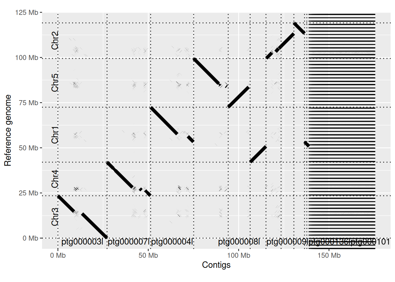
The following chunk imports the paf file and create a dotplot of contigs for line 1158 against the TAIR10 reference assembly, with contigs sorted by size.
library(pafr)
# Import the PAF file
path_to_paf <- "03_processing/05_genome_assembly/output/03_scaffolding/1158/tair10/ragtag.scaffold.asm.paf"
paf_file <- read_paf(path_to_paf)

# Plot contigs
dotplot(
  paf_file, label_seqs = TRUE, order_by='qstart',
  xlab = "Contigs", ylab = "Reference genome"
)

This looks pretty good. The direction of contigs is arbitrary, so it doesn’t matter that some are oriented backwards. You can see that most chromosomes are covered by a single, or a handful of contigs. This includes chromosome 4, which has an rDNA cluster which is usually very difficult to assemble. Chr2 also contains an rDNA cluster, and here the assembly splits into separate contigs. You can also see horizontal gaps corresponding to the centromeres. These are missing in the reference genome, but are well covered in the HiFi data.
On the right-hand side you can see a large number of horizontal stripes. These are fragments of <100kb that are mostly copies of the chloroplast genome, with some copies of rDNA and mitochondrial sequences.
Plot the scaffolded assembly
I used pannagram to plot scaffolded assemblies against a reference genome. Pannagram is a program for investigating structural variation between genomes. It is probably overkill if you only want to plot things, but it gives quite detailed plots and I knew I would need it later anyway.
Pannagram is in the alpha stage, so the commands could change, but I will outline how I did this.
Pannagram is intended to compare multiple genomes, and the first step is to put all the scaffolded assemblies you want to compare, including a reference genome if there is one, into a single directory that I will call fasta_dir.
In my case the contents of fasta_dir would contain files called
TAIR10_chr_all.fasta
1158.fasta
6024.fasta
6184.fasta
8249.fasta
The following command compares the genomes to a single reference genome - notice the absence of the .fasta suffix - and saves plots to outdir.
pannagram \
    -path_in fasta_dir \
    -path_out outdir \
    -ref TAIR10_chr_all \
    -cores 8 \
    -nchr 5
-cores tells the program to use 8 threads in parallel. -nchr tells the program to look only at the first five sequences. In this case that means the five autosomes, ignoring the chloroplast and mitochondrion.
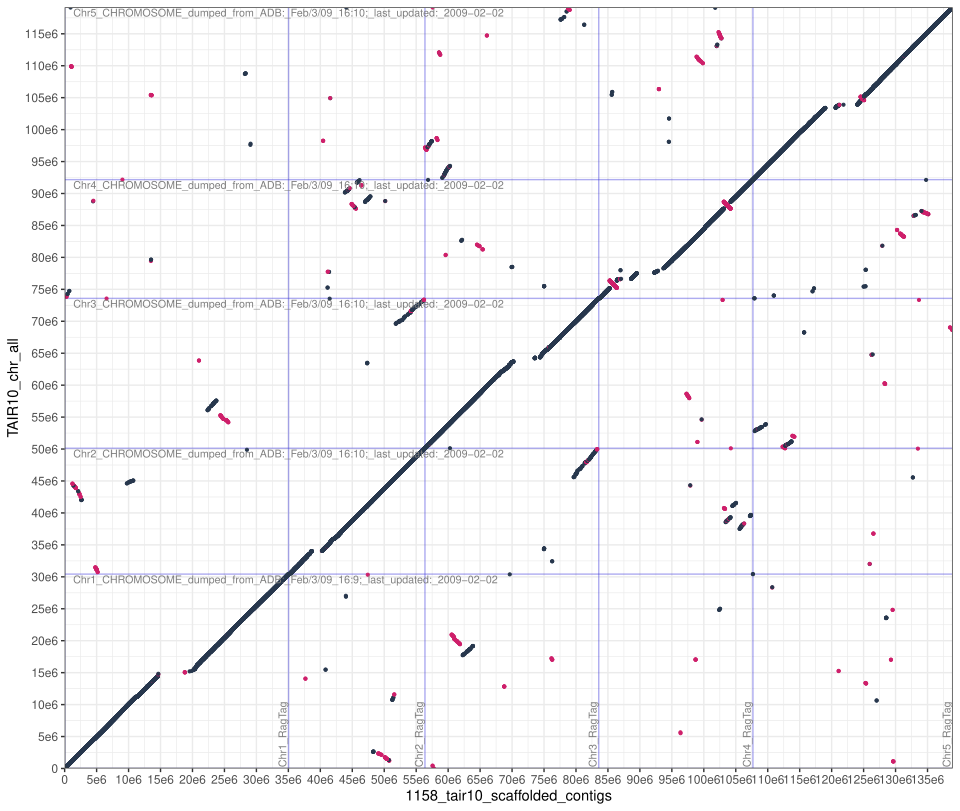
Here is an example of a dot plot for accession 1158. Red dots indicate reverse complement sequence.

We can see that the assembly looks essentially complete because there is a near unbroken line along the diagonal. Where there are breaks they are because the TAIR 10 reference genome does not have centromeres. You can also see regions homology between chromosomes all over the place, most obviously between the ends of chromosomes 2 and 3.

